Technical power details

Here we document the technical details behind GrowthBook power calculations and minimum detectable effect (MDE) calculations for both frequentist and Bayesian engines.

​

Frequentist engine details

​

Frequentist power

Below we describe technical details of our implementation. First we start with the definition of power. Power is the probability of a statistically significant result. We use the terms below throughout. Define:

1. the false positive rate as $\alpha$ (GrowthBook default is $\alpha=0.05$).
2. the critical values $Z_{1- \alpha / 2}= \Phi^{-1}(1-\alpha/2)$ and $Z_{1-\alpha}= \Phi^{-1}(1-\alpha)$ where $\Phi^{-1}$ is the inverse CDF of the standard normal distribution.
3. the true relative treatment effect as $\Delta$, its estimate as $\hat{\Delta}$ and its estimated standard error as $\hat{\sigma}_{\Delta}$. Note that as the sample size $n$ increases, $\hat{\sigma}_{\Delta}$ decreases by a factor of $1/\sqrt{n}$.

We make the following assumptions:

1. equal sample sizes across control and treatment variations. If unequal sample sizes are used in the experiment, use the smaller of the two sample sizes. This will produce conservative power estimates.
2. equal variance across control and treatment variations;
3. observations across users are independent and identically distributed;
4. all metrics have finite variance; and
5. you are running a two-sample t-test. If in practice you use CUPED, your power will be higher.

For a 1-sided test, the power is $$\begin{align} \pi = P\left(\frac{\hat{\Delta}}{\hat{\sigma}_{\Delta}} > Z_{1-\alpha}\right)=P\left(\frac{\hat{\Delta}-\Delta}{\hat{\sigma}_{\Delta}} > Z_{1-\alpha}-\frac{\Delta}{\hat{\sigma}_{\Delta}}\right)=1 - \Phi\left(Z_{1-\alpha}-\frac{\Delta}{\hat{\sigma}_{\Delta}}\right). \end{align}$$ For a 2-sided test (all GrowthBook tests are 2-sided), power is composed of the probability of a statistically significant positive result and a statistically significant negative result. Using the same algebra as in Equation 1 (except using $Z_{1-0.5\alpha}$ for the critical value), the probability of a statistically significant positive result is $$\begin{align} \pi_{pos} &= 1 - \Phi\left(Z_{1-\alpha/2}-\frac{\Delta}{\hat{\sigma}_{\Delta}}\right). \end{align}$$ The probability of a statistically significant negative result is $$\begin{align} \pi_{neg} &= P\left(\frac{\hat{\Delta}}{\hat{\sigma}_{\Delta}} < Z_{\alpha/2}\right)=P\left(\frac{\hat{\Delta}-\Delta}{\hat{\sigma}_{\Delta}} < Z_{\alpha/2}-\frac{\Delta}{\hat{\sigma}_{\Delta}}\right)=\Phi\left(Z_{\alpha/2}-\frac{\Delta}{\hat{\sigma}_{\Delta}}\right). \end{align}$$ For a 2-sided test, the power equals $$\begin{align} \pi = 1 - \Phi\left(Z_{1-\alpha/2}-\frac{\Delta}{\hat{\sigma}_{\Delta}}\right) + \Phi(Z_{\alpha/2} - \frac{\Delta}{\hat{\sigma}_{\Delta}}). \end{align}$$

​

Frequentist minimum detectable effect

Some customers want to know what effect size is required to produce at least $\pi$ power.
The minimum detectable effect is the smallest $\Delta$ for which nominal power (e.g., 80%) is achieved. Below we describe commonly used MDE calculations, though we do not use these at GrowthBook.
For a 1-sided test there is a closed form solution for the MDE. Solving Equation 1 for $\Delta$ produces $$\begin{align} \text{MDE} &= \hat{\sigma}_{\Delta}\left(\Phi^{-1}(1 - \alpha)-\Phi^{-1}(1 - \pi)\right). \end{align}$$ In the 2-sided case there is no closed form solution.
Often in practice the MDE is defined as the solution to inverting Equation 2.
This ignores the negligible term in Equation 3, and produces power estimates very close to $\pi$: $$\begin{align} \text{MDE}_{\text{two-sided}} &= \hat{\sigma}_{\Delta}\left(\Phi^{-1}(1 - \alpha/2)-\Phi^{-1}(1 - \pi)\right). \end{align}$$ This approach works when effects are defined on the absolute scale, where the uncertainty of effect estimate does not depend upon the true absolute effect. For relative inference, this does not hold, and so GrowthBook uses a different approach. The terms below are used to help define the variance of the sample lift.

1. Define $\Delta_{Abs}$ as the absolute effect.
2. Define $\mu_{A}$ as the population mean of variation $A$ and $\sigma^{2}$ as the population variance.
3. For variation $B$ analogously define $\mu_{B}$; recall that we assume equal variance across treatment arms.
4. Define $N$ as the per-variation sample size.
5. Define the sample counterparts as ($\hat{\mu}_{A}$, $\hat{\sigma}_{A}^{2}$, $\hat{\mu}_{B}$, and $\hat{\sigma}_{B}^{2}$).

Then the variance of the sample lift is $$\begin{align} \hat{\sigma}_{\Delta}^{2} &= \frac{\sigma^{2}}{N}\frac{1}{\mu_{A}^{2}} + \frac{\sigma^{2}}{N} *\frac{\mu_{B}^{2}}{\mu_{A}^{4}} \\&= \frac{\sigma^{2}}{N}\frac{1}{\mu_{A}^{2}} + \frac{\sigma^{2}}{N} *\frac{\left(\mu_{A}+\Delta_{Abs}\right)^{2}}{\mu_{A}^{4}}. \end{align}$$ Therefore, when inverting the power formula above to find the minimum $\Delta$ that produces at least 80% power, the uncertainty term $\hat{\sigma}_{\Delta}$ changes as $\Delta$ changes.
To find the MDE we solve for the equation below, where we make explicit the dependence of $\hat{\sigma}_{\Delta}$ on $\Delta$: $$\begin{align*} \frac{\Delta}{\hat{\sigma}_{\Delta}(\Delta)} = \Phi^{-1}\left({1-\alpha/2}\right) - \Phi^{-1}(1 - \pi). \end{align*}$$ Define the constant $k = \Phi^{-1}\left({1-\alpha/2}\right) - \Phi^{-1}(1 - \pi)$. We solve for $\mu_{B}$ in: $\frac{(\mu_{B}-\mu_{A})/\mu_{A}}{\sqrt{\text{Var}(\hat{\Delta})}} = k \iff (\mu_{B}-\mu_{A})^{2} =k^{2}\mu_{A}^{2}\text{Var}(\hat{\Delta}) = k^{2}\mu_{A}^{2}\left(\frac{\sigma^{2}}{N}\frac{1}{\mu_{A}^{2}} + \frac{\sigma^{2}}{N} *\frac{\mu_{B}^{2}}{\mu_{A}^{4}}\right).$ Rearranging terms shows that $\mu_{B}^{2}\left(1-\frac{\sigma^{2}}{N}\frac{k^{2}}{\mu_{A}^{2}}\right) + \mu_{B}\left(-2\mu_{A}\right) + \left(\mu_{A}^{2}-k^{2}\frac{\sigma^{2}}{N}\right) = 0.$ This is quadratic in $\mu_{B}$ and has solution $$\mu_{B} = \frac{2 \mu_{A} \pm \sqrt{4 \mu_{A}^{2}-4\left(1-\frac{\sigma^{2}}{N}\frac{k^{2}}{\mu_{A}^{2}}\right)\left(\mu_{A}^{2}-k^{2}\frac{\sigma^{2}}{N}\right)}}{2\left(1-\frac{\sigma^{2}}{N}\frac{k^{2}}{\mu_{A}^{2}}\right)} = \frac{\mu_{A} \pm \sqrt{\mu_{A}^{2}-\left(1-\frac{\sigma^{2}}{N}\frac{k^{2}}{\mu_{A}^{2}}\right)\left(\mu_{A}^{2}-k^{2}\frac{\sigma^{2}}{N}\right)}}{\left(1-\frac{\sigma^{2}}{N}\frac{k^{2}}{\mu_{A}^{2}}\right)} .$$ The discriminant reduces to $k^{2} * \frac{\sigma^{2}}{N} \left(1 - \frac{\sigma^{2}}{N} * \frac{k^{2}}{\mu_{A}^{2}}\right).$ so a solution for $\mu_{B}$ exists if and only if $$\begin{align} 2 - \frac{\sigma^{2}}{N} * \frac{k^{2}}{\mu_{A}^{2}} > 0 &\iff 2 > \frac{\sigma^{2}}{N} * \frac{k^{2}}{\mu_{A}^{2}} \iff N > \frac{\sigma^{2}k^{2}}{2\mu_{A}^{2}}. \end{align}$$ Similarly, the MDE returned can be negative if the denominator is negative, which is nonsensical.
We return cases only where the denominator is positive, which occurs if and only if: $$\begin{align} \left(1-\frac{\sigma^{2}}{N}\frac{k^{2}}{\mu_{A}^{2}}\right) > 0 \iff \left(1-\frac{\sigma^{2}}{N}\frac{k^{2}}{\mu_{A}^{2}}\right) > 0 \iff N > \frac{\sigma^{2}k^{2}}{\mu_{A}^{2}}. \end{align}$$ The condition in Equation 10 is stricter than the condition in Equation 9. In summary, there will be some combinations of $(\mu_{A}, \sigma_{2})$ where the MDE does not exist for a given $N$. If $\alpha=0.05$ and $\pi=0.8$, then $k\approx 2.8$. Therefore, a rule of thumb is that $N$ needs to be roughly 9 times larger than the ratio of the variance to the squared mean to return an MDE. In these cases, $N$ needs to be increased.

​

Sequential testing

To estimate power under sequential testing, we adjust the variance term $\hat{\sigma}_{\delta}$ to account for sequential testing, and then input this adjusted variance into our power formula. We assume that you look at the data only once, so our power estimate below is a lower bound for the actual power under sequential testing. Otherwise we would have to make assumptions about the temporal correlation of the data generating process. In sequential testing we construct confidence intervals as $$\begin{align*} \hat{\Delta} &\pm \hat{\sigma}*\sqrt{N} * \sqrt{\frac{2(N\rho^2 + 1)}{N^2\rho^2}\log\left(\frac{\sqrt{N\rho^2 + 1}}{\alpha}\right)} \end{align*}$$ where $\rho = \sqrt{\frac{-2\text{log}(\alpha) + \text{log}(-2 \text{log}(\alpha) + 1)}{N^*}}$ and $N^{\star}$ is a tuning parameter. This approach relies upon asymptotic normality. For power analysis we rewrite the confidence interval as $$\begin{align*} \hat{\Delta} &\pm \hat{\sigma}*\sqrt{N} * \sqrt{\frac{2(N\rho^2 + 1)}{N^2\rho^2}\log\left(\frac{\sqrt{N\rho^2 + 1}}{\alpha}\right)}\frac{Z_{1-\alpha/2}}{Z_{1-\alpha/2}} \\&=\hat{\Delta_{r}} \pm \tilde{\sigma}Z_{1-\alpha/2} \end{align*}$$ where $\tilde{\sigma} = \hat{\sigma}*\sqrt{N}\sqrt{\frac{2(N\rho^2 + 1)}{N^2\rho^2}\log\left(\frac{\sqrt{N\rho^2 + 1}}{\alpha}\right)}\frac{1}{Z_{1-\alpha/2}}$. We use power analysis described above, except we substitute $\tilde{\sigma}^{2}$ for $\hat{\sigma}_{\Delta}^{2}$.

​

Bayesian engine details

​

Bayesian power

For Bayesian power analysis, we let users specify the prior distribution of the treatment effect. We then estimate Bayesian power, which is the probability that the $(1 - \alpha)$ credible interval does not contain 0. We assume a conjugate normal-normal model, as follows: $$\begin{align*} \Delta &\stackrel{}{\sim}\mathcal{N}\left(\mu_{prior}, \sigma_{prior}^{2}\right) \\ \hat{\Delta}|\Delta &\stackrel{}{\sim}\mathcal{N}\left(\Delta, \hat{\sigma}_{\Delta}^{2}\right). \end{align*}$$ In words, the model has two parts: 1) the normal prior for the treatment effect, which is specified by you; and 2) conditional upon the treatment effect, the estimated effect is normally distributed. The normal prior has several advantages, including: 1) bell-shaped distribution around the prior mean, so that extreme estimates will be shrunk more towards the prior than moderate estimates; 2) the ability to specify two moments, which is often the right amount of information for a prior; and 3) simplicity.
The conditional normality of the effect estimate is motivated by the central limit theorem. We use the normal distribution below to approximate the posterior: $$\begin{align*} \Delta|\hat{\Delta} &\stackrel{}{\sim}\mathcal{N}\left(\Omega^{-1}\omega, \Omega^{-1}\right) \\\Omega &= 1/\sigma_{prior}^{2} + 1/\hat{\sigma}_{\Delta}^{2} \\\omega &= \mu_{prior}/\sigma_{prior}^{2} + \hat{\Delta}/\hat{\sigma}_{\Delta}^{2}. \end{align*}$$ This is an approximation to the posterior because $\Delta$ affects $\hat{\sigma}_{\Delta}^{2}$. We tested this approximation through extensive simulations, and found it had comparable coverage and mean squared error to a posterior distribution empirically sampled using Metropolis Hastings. We define rejection as the $100(1-\alpha)$% confidence interval not containing zero.
For our posterior approximation, this occurs if the posterior mean for $\Delta|\hat{\Delta}$ (i.e., $\Omega^{-1}\omega$) divided by its posterior standard deviation$\left(\text{i.e., }\sqrt{\Omega^{-1}}\right)$ is beyond the the appropriate critical threshold $Z^{\star}$ (e.g., $\Phi^{-1}(0.975)$ for $\alpha=0.05$). Inside of a Bayesian framework, it can help to permit the case where the prior model is misspecified.
That is, the prior specified by the customer differs from the true prior that generates the treatment effect.
We permit misspecification of the prior for $\Delta$, as we assume that the true data generating process (DGP) is $\Delta \stackrel{}{\sim}\mathcal{N}\left(\mu_{\star}, \sigma_{\star}^{2}\right)$, while the specified DGP has $\Delta \stackrel{}{\sim}\mathcal{N}\left(\mu_{prior}, \sigma_{prior}^{2}\right)$. We assume the prior is specified on the relative scale. In derivations below we use the marginal distribution of $\hat{\Delta}$, which we find using its moment generating function: $$\begin{align*} E\left[\exp^{t\hat{\Delta}}\right] &= E_{\Delta}\left[E\left[\exp^{t\hat{\Delta}}|\Delta\right]\right] \\&= E_{\Delta}\left[\exp^{t\Delta + t^{2}\hat{\sigma}_{\Delta}^{2}}\right] \\&= \exp^{ t^{2}\hat{\sigma}_{\Delta}^{2}}E_{\Delta}\left[\exp^{t\Delta}\right]\ \\&= \exp^{ t^{2}\hat{\sigma}_{\Delta}^{2}}\exp^{t\mu^{\star} + t^{2}\sigma_{\star}^{2}} \\&\stackrel{}{\sim}\mathcal{N}\left(\mu^{\star}, \sigma_{\star}^{2}+\hat{\sigma}_{\Delta}^{2}\right). \end{align*}$$ For a 2-sided test the probability of rejection is $$\begin{align*} &P\left(\left|\frac{\Omega^{-1}\omega}{\Omega^{-1/2}}\right| > Z_{1-\alpha/2}\right) \\&=P\left(\left|\left(\frac{1}{\sigma_{prior}^{2}} + \frac{1}{\hat{\sigma}_{\Delta}^{2}}\right)^{-1/2} \left(\frac{\mu_{prior}}{\sigma_{prior}^{2}} + \frac{\hat{\Delta}}{\hat{\sigma}_{\Delta}^{2}}\right)\right|> Z_{1-\alpha/2}\right) \\&= P\left(\left|\left(\frac{\mu_{prior}}{\sigma_{prior}^{2}} + \frac{\hat{\Delta}}{\hat{\sigma}_{\Delta}^{2}}\right)\right|> \left(\frac{1}{\sigma_{prior}^{2}} + \frac{1}{\hat{\sigma}_{\Delta}^{2}}\right)^{1/2} Z_{1-\alpha/2}\right) \\&=P\left(\left(\frac{\mu_{prior}}{\sigma_{prior}^{2}} + \frac{\hat{\Delta}}{\hat{\sigma}_{\Delta}^{2}}\right)> \left(\frac{1}{\sigma_{prior}^{2}} + \frac{1}{\hat{\sigma}_{\Delta}^{2}}\right)^{1/2} Z_{1-\alpha/2}\right) \\&+ P\left(\left(\frac{\mu_{prior}}{\sigma_{prior}^{2}} + \frac{\hat{\Delta}}{\hat{\sigma}_{\Delta}^{2}}\right)< -\left(\frac{1}{\sigma_{prior}^{2}} + \frac{1}{\hat{\sigma}_{\Delta}^{2}}\right)^{1/2} Z_{1-\alpha/2}\right) \\&= P\left(\hat{\Delta}> \hat{\sigma}_{\Delta}^{2}\left[\left(\frac{1}{\sigma_{prior}^{2}} + \frac{1}{\hat{\sigma}_{\Delta}^{2}}\right)^{1/2} Z_{1-\alpha/2} - \frac{\mu_{prior}}{\sigma_{prior}^{2}}\right]\right) \\&+ P\left(\hat{\Delta}< -\hat{\sigma}_{\Delta}^{2}\left[\left(\frac{1}{\sigma_{prior}^{2}} + \frac{1}{\hat{\sigma}_{\Delta}^{2}}\right)^{1/2} Z_{1-\alpha/2} + \frac{\mu_{prior}}{\sigma_{prior}^{2}}\right]\right) \\&= P \left( \frac{\hat{\Delta}-\mu_{\star}}{\sqrt{\hat{\sigma}_{\Delta}^{2}+\sigma_{\star}^{2}}}> \frac{\hat{\sigma}_{\Delta}^{2}\left[\left(\frac{1}{\sigma_{prior}^{2}} + \frac{1}{\hat{\sigma}_{\Delta}^{2}}\right)^{1/2} Z_{1-\alpha/2} - \frac{\mu_{prior}}{\sigma_{prior}^{2}}\right]-\mu_{\star}}{\sqrt{\hat{\sigma}_{\Delta}^{2}+\sigma^{2}_{\star}}}\right) \\&+ P\left(\frac{\hat{\Delta}-\mu_{\star}}{\sqrt{\hat{\sigma}_{\Delta}^{2}+\sigma_{\star}^{2}}}< \frac{-\hat{\sigma}_{\Delta}^{2}\left[\left(\frac{1}{\sigma_{prior}^{2}} + \frac{1}{\hat{\sigma}_{\Delta}^{2}}\right)^{1/2} Z_{1-\alpha/2} + \frac{\mu_{prior}}{\sigma_{prior}^{2}}\right]-\mu_{\star}}{\sqrt{\hat{\sigma}_{\Delta}^{2}+\sigma_{\star}^{2}}}\right) \\&= 1-\Phi\left(\frac{\hat{\sigma}_{\Delta}^{2}\left[\left(\frac{1}{\sigma_{prior}^{2}} + \frac{1}{\hat{\sigma}_{\Delta}^{2}}\right)^{1/2} Z_{1-\alpha/2} - \frac{\mu_{prior}}{\sigma_{prior}^{2}}\right]-\mu_{\star}}{\sqrt{\hat{\sigma}_{\Delta}^{2}+\sigma^{2}_{\star}}}\right) \\&+ \Phi\left(\frac{-\hat{\sigma}_{\Delta}^{2}\left[\left(\frac{1}{\sigma_{prior}^{2}} + \frac{1}{\hat{\sigma}_{\Delta}^{2}}\right)^{1/2} Z_{1-\alpha/2} + \frac{\mu_{prior}}{\sigma_{prior}^{2}}\right]-\mu_{\star}}{\sqrt{\hat{\sigma}_{\Delta}^{2}+\sigma_{\star}^{2}}}\right). \end{align*}$$ In practice GrowthBook assumes there is a true fixed effect size, i.e., the variance of the data generating process $\sigma_{\star}^{2}$ equals 0, and $\mu_{\star} = \Delta$, so two-sided power is $$\begin{align} \begin{split} \pi &= 1-\Phi\left( \frac{ \hat{\sigma}_{\Delta}^{2}\left[\left(\frac{1}{\sigma_{prior}^{2}} + \frac{1}{\hat{\sigma}_{\Delta}^{2}}\right)^{1/2} Z_{1-\alpha/2} - \frac{\mu_{prior}}{\sigma_{prior}^{2}}\right]-\Delta} {\sqrt{\hat{\sigma}_{\Delta}^{2}}} \right) \\&+\Phi\left( \frac{ -\hat{\sigma}_{\Delta}^{2}\left[\left(\frac{1}{\sigma_{prior}^{2}} + \frac{1}{\hat{\sigma}_{\Delta}^{2}}\right)^{1/2} Z_{1-\alpha/2} - \frac{\mu_{prior}}{\sigma_{prior}^{2}}\right]-\Delta} {\sqrt{\hat{\sigma}_{\Delta}^{2}}} \right) . \end{split} \end{align}$$ We assume that $\sigma_{\star}^{2}=0$ for simplicity and because large values of $\sigma_{\star}^{2}$ can result in negative MDEs (see here). If the prior variance $\sigma_{prior}^{2}$ equals infinity then Equation 11 reduces to Equation 4.

​

Bayesian minimum detectable effect

MDEs are not well defined in the Bayesian literature. We provide MDEs in Bayesian power analysis for customers that are used to conceptualizing MDEs and want to be able to leverage prior information in their analysis. We could define the MDE as the minimum value of $\mu_{\star}$ such that at least $\pi$ power is achieved. This definition is Bayesian in that it permits uncertainty in the parameters in the data generating process. However, if $\sigma_{\star}^{2}$ is large, then there are some combinations of parameters where the MDE can be negative. That is, negative values of $\mu_{\star}$ result in power being at least $\pi$. Usually the inferential focus is the true treatment effect for the experiment ($\Delta$), not the population mean from which $\Delta$ is just one realization ($\mu_{\star}$), so we set $\sigma_{\star}^{2} = 0$ and consequently, $\Delta = \mu_{\star}$. This is why in practice we frame our Bayesian MDE as, “given our prior beliefs and the data generating process, what is the probability we can detect an effect of size $\Delta$?”, where $\Delta$ is a fixed number. Another subtlety is that for a fixed sample size, Equation 11 can be decreasing in effect size, illustrated by Figure 1.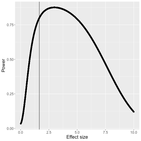 Figure 1 shows the case where the group sample sizes are 1500, the data mean is 0.1, the data variance is 0.5, the specified prior mean $\mu_{prior} = 0.1$, the specified prior variance $\sigma_{prior}^{2}$ is 0.3, and the variance of the data generating process $\sigma_{\star}^{2}$ is 0. Nominal 80% power occurs at 1.65, continues to increase in effect size until the effect size is about 3, and then begins decreasing. Power decreases in effect size because the variance in Equation 8 is quadratic in effect size, and in Equation 11 the term in front of $Z_{1-\alpha/2}$ goes to infinity as $\Delta$ gets large. The coefficient in front of $Z_{1-\alpha/2}$ in Equation 4 is 1, so frequentist power is increasing in effect size in all cases. Monotonicity does hold for Bayesian power for absolute effects, where the variance is not affected by the effect size. Because power is not monotonic in effect size, we perform a grid search across effect sizes ranging from 0 to 500%. The derivative of Equation 11 is bounded in absolute value by $2 \phi(0) < 0.8$, where $\phi(.)$ is the density of the standard normal distribution. Let the length of one grid cell equal $l$. We evaluate power at the points $\left\{0, l, 2l, ..., 5 -l , 5\right\}.$ Suppose the power at the $k^{\text{th}}$ gridpoint is $\pi_{k}$, $k>0$. Because 1) the maximum slope from the midpoint to the endpoint of the cell is no greater than $2 \phi(0)$; and 2) the maximum distance from where power is evaluated is $l/2$, the maximum power in $\left[(l-1)k, lk \right]$ is no greater than $\max\left(\pi_{k-1}, \pi_{k}\right)+\phi(0)l$. Motivated by this fact, we describe our approach in Algorithm 1. In words, Algorithm 1 evaluates power at $\Delta=\left\{0, 0.001, 0.002, ... 5\right\}$, until it finds the first element $k$ such that $\pi(k) >= \pi - \phi(0)l$. If power exceeds this threshold, then we evaluate a finer grid across the range from $[k-l, k]$, where the grid cell length is $l' << l$. We find the first element (if it exists) of this finer grid where power is at least $\pi$. We return this first element as the solution if it exists; otherwise we keep searching the coarse grid. Algorithm 1

1. Define $l$ as the length between points at which power is evaluated (l=0.001 in production).
2. Define the grid of points between 0 and 5 as $\mathcal{G} = \left\{0, l, 2l, ..., 5 -l , 5\right\}.$
3. Begin evaluating $\pi(k)$ for $k \in \mathcal{G}$.
4. If $\pi(k) < \pi - \phi(0)l$ for all $k$, then the MDE does not exist. Otherwise:
5. Find the first $k \in \mathcal{G}$ such that $\pi(k) >= \pi - \phi(0)l$. Define $l'$ as a finer grid resolution (in production, $l' = l / 100$). Find the first element of the set $\left\{k -1, k-1+l', k-1+2l', ..., k-l', k \right\}$ such that power evaluated at that point is at least $\pi$. If no such point exists, return to the coarser grid search in Step 3.

If power exceeds $\pi + \phi(0)l'$ at any point in $[0, 5]$, then Algorithm 1 is guaranteed to detect it. In practice we use $l=10^{-3}$ and $l'=10^{-5}$.